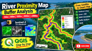
I have prepared the River Proximity Map for the Buffer 250m, 500m, 1000m, 2000m and beyond 2000m for the study area. I used the Sentinel 2 satellite image 10m Resolution of Band Green and Near Infrared for the calculation of NDWI. Satellite Image Link.
Tutorial Video Link: Step By Step Part 1
Hands-On QGIS Practical
River Proximity Map for Flood Risk Assessment Using Sentinel-2 Imagery
A complete click-by-click practical exercise: Sentinel-2 → NDWI → River Extraction → Proximity Analysis → Flood Susceptibility Classes → Map Layout → Export
1. Practical Objectives
- Load Sentinel-2 imagery into QGIS.
- Create and interpret a water index (NDWI).
- Extract the main river from Sentinel-2 imagery.
- Create river-based proximity zones using buffer analysis.
- Assign flood-proximity susceptibility classes.
- Clip and symbolize the final analysis.
- Create a professional QGIS map layout.
- Export the final map as PNG and PDF.
2. Prepare the Project Folder
Before opening QGIS, create the following folder structure to keep all data organized:
Flood_Proximity_Project/
01_Raw_Data/Sentinel2/
01_Raw_Data/Boundary/
02_Processed_Data/Raster/
02_Processed_Data/Vector/
03_Output/Maps/
03_Output/Tables/
04_QGIS_Project/
Open QGIS and immediately save the project using Project → Save As. Suggested name: River_Proximity_Flood_Risk.qgz.
3. Start QGIS and Set the Project CRS
- Open QGIS and create a new project.
- Check the CRS shown in the bottom-right corner.
- Click the CRS indicator and select an appropriate projected CRS for your study area.
- Click Apply → OK.
Important: Proximity and buffer distances should be calculated in a projected CRS with metre units. Do not rely on geographic coordinates (degrees) for metre-based distance analysis.
4. Add the Study Area Boundary
- Click Layer → Add Layer → Add Vector Layer.
- Browse to the study area boundary file and click Add.
- Right-click the layer → Properties → Information to check its CRS.
- If necessary, reproject it using Right-click → Export → Save Features As and select an appropriate projected CRS.
- Save the reprojected boundary as Study_Area.gpkg.
5. Add Sentinel-2 Bands
For the NDWI calculation, load the following Sentinel-2 Level-2A bands:
| Band | Name | Resolution | Purpose |
| B03 | Green | 10 m | Water detection / NDWI |
| B08 | Near Infrared (NIR) | 10 m | Water detection / NDWI |
| B04 | Red | 10 m | Optional visual composite |
- Click Layer → Add Layer → Add Raster Layer.
- Select B03 and B08.
- Click Add → Close.
- Confirm that both layers align correctly.
6. Optional: Create a False Color Composite
A False Color Composite helps visually identify rivers and other land-cover features. A common Sentinel-2 combination is:
| Display Channel | Band |
| Red | B08 (NIR) |
| Green | B04 (Red) |
| Blue | B03 (Green) |
Water generally appears dark, while healthy vegetation commonly appears reddish. Use this as visual support; the actual water extraction will use NDWI.
7. Calculate NDWI
NDWI (Normalized Difference Water Index) is calculated as:
NDWI = (Green − NIR) / (Green + NIR)
- Click Raster → Raster Calculator.
- Insert the exact B03 and B08 layer names from the layer list.
- Use the expression below.
- Choose the output location: 02_Processed_Data/Raster/NDWI.tif.
- Click OK / Run.
(“B03@1” – “B08@1”) / (“B03@1” + “B08@1”)
Note: Replace B03 and B08 with the exact raster names shown in your QGIS project if necessary.
8. Inspect the NDWI Result
- Right-click NDWI → Properties → Symbology.
- Select Singleband Pseudocolor.
- Click Classify and then Apply → OK.
- Use the Identify Features tool to click river, vegetation, settlement, and other surfaces.
- Compare the NDWI values and identify a suitable water threshold.
Higher positive NDWI values generally indicate water, but the correct threshold should be checked for the specific image and study area.
9. Create a Water Mask
- Open Raster → Raster Calculator.
- Start by testing a threshold such as NDWI > 0.
- Save the output as Water_Mask.tif.
- Inspect the result and adjust the threshold if necessary.
Example expression: (“NDWI@1” > 0)
Possible alternative thresholds for testing include NDWI > 0.1 or NDWI > 0.2. Choose the threshold that best separates the actual river from surrounding land.
10. Polygonize the Water Mask
- Open Processing → Toolbox.
- Search for Polygonize (Raster to Vector).
- Set Input raster = Water_Mask.tif.
- Set Field name = DN.
- Save the result as Water_Polygons.gpkg.
- Click Run.
The resulting polygons normally include both water and non-water classes.
11. Extract Water Polygons
- Open the attribute table of Water_Polygons.
- Click Select Features by Expression.
- Use the expression: “DN” = 1.
- Click Select Features.
- Right-click the layer → Export → Save Selected Features As.
- Save the output as Water_Only.gpkg.
12. Extract the Main River
- Turn on the Sentinel-2 image or False Color Composite as a reference.
- Zoom to the main river.
- Use the Select Features tool to select the river polygon or polygons.
- Hold Ctrl if multiple disconnected polygons must be selected.
- Right-click Water_Only → Export → Save Selected Features As.
- Save the result as Main_River.gpkg.
Check the extracted river carefully. Ponds, lakes, wetlands, and temporary water bodies may also be detected by NDWI.
13. Define River Proximity Classes
| Zone | Distance from River | Flood Proximity Susceptibility | Example Score |
| 1 | 0–250 m | Very High | 5 |
| 2 | 250–500 m | High | 4 |
| 3 | 500–1,000 m | Moderate | 3 |
| 4 | 1,000–2,000 m | Low | 2 |
| 5 | More than 2,000 m | Very Low | 1 |
These distances are suitable as a teaching example. For scientific research, distance thresholds should be justified using local flood history, river morphology, hydrology, and other evidence.
14. Create the 250 m Buffer
- Open Processing Toolbox and search for Buffer.
- Set Input layer = Main_River.
- Set Distance = 250 metres.
- Set Segments = 5 or use the default value.
- Enable Dissolve result if appropriate.
- Save as Buffer_250m.gpkg.
- Click Run.
15. Create the Remaining Buffers
Repeat the Buffer tool for the following distances:
| Buffer | Output File |
| 500 m | Buffer_500m.gpkg |
| 1,000 m | Buffer_1000m.gpkg |
| 2,000 m | Buffer_2000m.gpkg |
At this stage the buffers overlap. The next step creates separate, non-overlapping distance rings.
16. Create Non-Overlapping Distance Rings
Open Processing Toolbox and search for Difference. Create the following zones:
| Input Layer | Overlay Layer | Output |
| Buffer_500m | Buffer_250m | Zone_250_500m.gpkg |
| Buffer_1000m | Buffer_500m | Zone_500_1000m.gpkg |
| Buffer_2000m | Buffer_1000m | Zone_1000_2000m.gpkg |
The 0–250 m zone is simply the Buffer_250m layer.
17. Create the Area Beyond 2 km
- Open Processing Toolbox → Difference.
- Set Input layer = Study_Area.
- Set Overlay layer = Buffer_2000m.
- Run the tool.
- Save the result as Zone_Over_2000m.gpkg.
This represents the Very Low proximity class within the study area.
18. Add Risk Attributes
For each proximity zone, open the Attribute Table and click Toggle Editing → Field Calculator.
- Create a new whole-number field named Risk_Score.
- Assign values from 5 (Very High) to 1 (Very Low).
- Create a text field named Risk_Class.
- Assign the appropriate class name.
| Distance | Risk Score | Risk Class |
| 0–250 m | 5 | Very High |
| 250–500 m | 4 | High |
| 500–1,000 m | 3 | Moderate |
| 1,000–2,000 m | 2 | Low |
| >2,000 m | 1 | Very Low |
19. Merge the Proximity Zones
- Open Processing Toolbox.
- Search for Merge Vector Layers.
- Select all five proximity zones.
- Choose a GeoPackage output.
- Save as River_Proximity_Risk.gpkg.
- Click Run.
20. Clip the Final Analysis to the Study Area
- Open Processing Toolbox → Clip.
- Input layer = River_Proximity_Risk.
- Overlay layer = Study_Area.
- Save as Final_River_Proximity_Risk.gpkg.
- Click Run.
This ensures that no analysis polygons extend outside the study boundary.
21. Symbolize the River Proximity Map
- Right-click Final_River_Proximity_Risk → Properties → Symbology.
- Select Categorized.
- Select Risk_Class as the classification field.
- Click Classify.
- Arrange the classes in the logical order: Very Low → Low → Moderate → High → Very High.
- Click Apply → OK.
Keep Main_River above the proximity zones in the Layers Panel so that the river remains clearly visible.
22. Create the Final Print Layout
- Click Project → New Print Layout.
- Enter a layout name such as River_Proximity_Map.
- Click OK.
- Select Add Item → Add Map and draw the main map frame.
- Adjust the extent and scale using Item Properties.
23. Add Essential Map Elements
- Map title: River Proximity-Based Flood Susceptibility Map of [Study Area]
- Legend showing the five susceptibility classes and the river
- Scale bar
- North arrow
- Study area boundary
- Data source information
- Projection / CRS information
- Optional inset location map
Example source note: Data Source: Sentinel-2 MSI imagery and study area boundary. Analysis: NDWI-based river extraction and distance proximity analysis. Software: QGIS.
24. Add an Optional Inset Location Map
- Add a second, smaller map using Add Item → Add Map.
- Set its extent to show the broader region, district, or Bangladesh.
- Display the study area prominently.
- Add a simple border and a short location label if needed.
25. Final Quality-Control Checklist
☐ The extracted river matches the actual river visible in Sentinel-2 imagery.
☐ All buffers were created in metres using a projected CRS.
☐ Distance zones do not overlap.
☐ The legend matches the risk classes shown on the map.
☐ The study area boundary is clearly visible.
☐ Labels and map elements are readable.
☐ The map title clearly describes the analysis.
☐ The data source and CRS are included.
☐ The final map has been checked at the intended print size.
26. Export the Final Map
- In the Layout window, click Layout → Export as Image.
- Select PNG for reports and presentations.
- Use approximately 300 DPI for high-quality output.
- Save as River_Proximity_Flood_Risk_Map.png.
- For a printable report, click Layout → Export as PDF.
- Save as River_Proximity_Flood_Risk_Map.pdf.
27. Complete Workflow Summary
Sentinel-2 Level-2A imagery
↓
Load B03 (Green) and B08 (NIR)
↓
Calculate NDWI
↓
Inspect values and select a water threshold
↓
Create Water Mask
↓
Polygonize raster
↓
Extract Main River
↓
Create 250, 500, 1,000 and 2,000 m buffers
↓
Create non-overlapping distance rings
↓
Assign proximity susceptibility scores
↓
Merge and clip to the study area
↓
Apply symbology
↓
Create Print Layout
↓
Export PNG and PDF
28. Important Scientific Note
River proximity is an important flood-susceptibility factor, but distance from a river alone does not represent complete flood risk. A comprehensive flood-risk or flood-susceptibility assessment may also include elevation, slope, rainfall, drainage density, land use/land cover, soil characteristics, historical flood extent, and exposure/vulnerability. For advanced research, the river-proximity layer can be standardized and combined with other factors using a justified weighting approach such as AHP or another multi-criteria decision method.